PWR-HYBRID-3/reachability/WALKTHROUGH.md

Linear Reach Analysis — Walkthrough

Status: preliminary example for the HAHACS thesis, not a final safety proof. The linear-reach artifacts in this directory use linearization of a nonlinear plant, which means every safety claim here is approximate, not sound. The follow-on nonlinear reach (via ReachabilityAnalysis.jl) will close that gap.

This document is a self-contained walkthrough of what got built, what it proves, and where it falls short. Read it cold; you shouldn't need the conversation transcript.

Contents

1. The per-mode reach-obligation taxonomy
2. Mode boundary definitions (entry / exit / time budgets)
3. Code walkthrough: how each artifact works
4. Results: what's proven, what isn't
5. Caveats, gaps, and next steps

---

1. The per-mode reach-obligation taxonomy

The controller has four DRC modes. They are not all reach-analyzed the same way. Two fundamentally different reach obligations apply:

• Equilibrium modes (q_shutdown, q_operation) — the plant is parked at some setpoint. The obligation is forever-invariance: does the state stay in the safe set under bounded disturbance?
• Transition modes (q_heatup, q_scram) — the plant is being driven from one mode's territory to another's. The obligation is reach-avoid: from X_entry, reach X_exit within a bounded time budget [T_min, T_max], maintaining inv_holds along the way. There is essentially no external disturbance in these modes.

The whole point of doing per-mode reach is not generic disturbance rejection — it's to prove that the DRC's discrete transitions (which ltlsynt guarantees at the discrete level) actually fire in physical time on the real plant. The reach artifact is what transfers discrete correctness to physical correctness. If q_heatup's reach set never enters t_avg_in_range ∧ p_above_crit ∧ inv1_holds, the DRC is written against a transition that can't physically happen, and the hybrid composition is broken.

Taxonomy table

Mode	X_entry	X_safe (along trajectory)	X_exit or goal	T_max
shutdown (eq.)	q_shutdown at DRC init (n small, T near T_standby)	inv_shutdown_holds (TBD)	t_avg_above_min	—
heatup (trans.)	X_exit(shutdown)	inv1_holds (fuel + rate + subcooling)	t_avg_in_range ∧ p_above_crit ∧ inv1_holds	5 hr
operation (eq.)	X_exit(heatup)	inv2_holds (trip avoidance)	stays forever OR ¬inv2_holds → scram	—
scram (trans.)	X_exit(operation) ∪ X_exit(heatup) (either can scram)	inv_scram_holds — n monotone non-increasing	n ≤ 1e-4	60 s

Formal claim per mode

Example for heatup:

Given x(0) ∈ X_entry(heatup),
applying u = ctrl_heatup(t, x, plant, ref),
with Q_sg = 0 (no external disturbance),
and α ∈ α_nominal [optionally: · (1 ± δ)],
we show ∃ T ∈ [T_min, T_max] such that:
  x(T) ∈ X_exit(heatup)                      [reach]
  x(t) ∈ inv1_holds   ∀t ∈ [0, T]           [avoid]

Operation mode is structurally different — no explicit T, obligation is forever-invariance under disturbance:

Given x(0) ∈ X_entry(operation),
applying u = ctrl_operation_lqr(x),
with Q_sg ∈ [w_lo, w_hi],
we show x(t) ∈ inv2_holds ∀t ≥ 0.

---

2. Mode boundary definitions

Concretized in predicates.json under mode_boundaries. Values are engineering-reasonable-but-made-up for this preliminary demo; they are not calibrated to a specific plant's tech specs. Final thesis defense will require real tech-spec numbers.

q_shutdown (equilibrium)

• X_entry: n ∈ [1e-7, 1e-4], T_f = T_c = T_cold ∈ [270, 280] °C
• X_safe: TBD — conservative: stay near T_standby = 275 °C with n subcritical
• X_exit: T_c ≥ T_standby + 5.556 (operator has warmed the coolant above the t_avg_above_min threshold)
• T_max: none (equilibrium mode)

q_heatup (transition)

• X_entry: n ∈ [5e-4, 5e-3], T_f ∈ [275, 295], T_c ∈ [281, 295], T_cold ∈ [270, 281]. "Operator has warmed coolant past t_avg_above_min and pulled rods toward criticality."
• X_safe = inv1_holds: fuel centerline ≤ 1200 °C, T_cold subcooled, |dT_c/dt| ≤ 50 °C/hr (tech-spec 28 °C/hr + overshoot budget).
• X_exit = t_avg_in_range ∧ p_above_crit ∧ inv1_holds: T_c ∈ [T_c0 ± 2.78], n ≥ 1e-4, all inv1 halfspaces.
• T_max = 5 hours = 18000 s. Rationale: tech-spec 28 °C/hr over a 60 °F (33.3 °C) span is 1.19 hr nominal; 4× margin.
• T_min = 2 hr 8.6 min = 7714 s. Physical floor: heatup faster than 28 °C/hr violates the rate invariant; accounting for non-uniform ramp, can't exceed ~1/1.3 × the tech-spec time.

q_operation (equilibrium)

• X_entry = X_exit(heatup)
• X_safe = inv2_holds: fuel limit, T_c high/low trip, n high/low, cold-leg subcooled. Conjunction of 6 halfspaces.
• Disturbance: Q_sg ∈ [0.85, 1.00] · P_0 (grid load-follow envelope; could tighten to ±5% steady-state or widen to ±30% for aggressive load-following).
• T_max: none (equilibrium mode).

q_scram (transition)

• X_entry: any state where inv1_holds or inv2_holds fails.
• X_safe: n'(t) ≤ 0 (monotone non-increasing power) AND temperatures bounded.
• X_exit: n ≤ 1e-4.
• T_max = 60 s. Rationale: NRC requires subcritical within seconds; 60 s is generous for our lumped model with idealized rod insertion.

---

3. Code walkthrough

Files in reachability/ and what each does.

predicates.json

Single source of truth for all predicate concretizations. Three categories:

• operational_deadbands — soft bands used by the DRC for mode transitions (t_avg_above_min, t_avg_in_range, p_above_crit).
• safety_limits — hard one-sided halfspaces for physical damage mechanisms and trip setpoints (fuel_centerline, t_avg_high_trip, t_avg_low_trip, n_high_trip, n_low_operation, cold_leg_subcooled, heatup_rate_upper, heatup_rate_lower).
• mode_invariants — inv1_holds, inv2_holds as conjunctions of safety_limits.

Plus mode_boundaries (entry/exit/time budgets per mode, as above).

load_predicates.m

Reads the JSON, resolves rhs_expr strings (which reference plant-derived constants like T_c0, T_cold0, T_standby) into numeric bounds, and returns a pred struct. Key entries:

pred.constants                 % T_c0, T_f0, T_cold0, T_standby, etc.
pred.operational_deadbands     % struct of (A_poly, b_poly, meaning)
pred.safety_limits             % same
pred.mode_invariants.inv1_holds    % conjunction of safety_limits
pred.mode_invariants.inv2_holds    % conjunction of safety_limits

Each A_poly is an n_halfspaces x 10 matrix; each b_poly is n_halfspaces x 1. The predicate is {x : A_poly * x ≤ b_poly}.

pke_linearize.m (in plant-model/)

Numerical Jacobians via central finite differences at any (x_star, u_star, Q_star). Returns (A, B, B_w) such that for small perturbations dx, du, dw:

dx/dt ≈ A dx + B du + B_w dw,    w = Q_sg

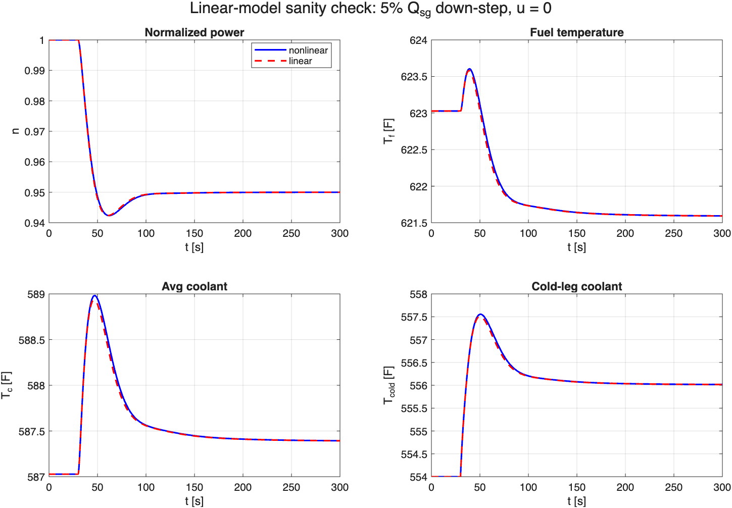
Validated in plant-model/test_linearize.m: under a 5% Q_sg step at u=0, the linear model matches the nonlinear sim to ~4e-4 relative error at 60 s, improving to 5e-6 at 300 s.

Eigenvalue check at the operating point:

max Re(eig) = -0.0124    (slowest mode: thermal loop)
min Re(eig) = -65.93     (fastest mode: delayed-neutron precursor)
stiffness ratio ≈ 5000

See docs/figures/linearize_sanity.png:

reach_linear.m

~50 lines. Propagates a box over-approximation of the reach tube for a linear system dx/dt = A_cl·x + B_w·w, with x(0) in a box and w in an interval.

The analytic solution is:

x(t) = e^(A·t) x(0) + ∫₀ᵗ e^(A·(t-s)) B_w w(s) ds

Per-step propagation:

A_step = expm(A_cl * dt);                  % state transition
G_step = [integral of e^(A·s) B_w  ds from 0 to dt]  % via augmented matrix trick

x_center  <- A_step * x_center              % signed
halfwidth <- |A_step| * halfwidth           % elementwise abs, sound box bound

S_center  <- A_step * S_center + G_step * w_mid
S_half    <- |A_step| * S_half + |G_step| * w_half

The |A_step| elementwise abs is the key soundness ingredient. A box |dx| ≤ h under a linear map M·dx is bounded axis-by-axis by |M|·h. Without the elementwise abs, signed positive/negative contributions cancel spuriously and you undercount — spotted this bug the first time I ran the tube and it came out suspiciously tight.

G_step is computed exactly via the Van Loan (1978) augmented-matrix trick:

M_aug = expm([A_cl, B_w; zeros(1, n+1)] * dt);
G_step = M_aug(1:n, n+1);   % upper-right block IS the integral

reach_operation.m

End-to-end operation-mode reach. Pipeline:

plant = pke_params();
x_op  = pke_initial_conditions(plant);
pred  = load_predicates(plant);
[A, B, B_w] = pke_linearize(plant);

Q_lqr = diag([1, 1e-3,..., 1e2, 1]);       % same as ctrl_operation_lqr
R_lqr = 1e6;
K     = lqr(A, B, Q_lqr, R_lqr);
A_cl  = A - B*K;                           % LQR-shaped closed loop

delta_entry = [0.01*n_op; 0.001*|C_i_op|; 0.1; 0.1; 0.1];
W = [0.85*P_0, 1.00*P_0];                  % disturbance envelope
tspan = [0, 600];

[T, R_lo, R_hi, center] = reach_linear(A_cl, B_w, zeros(10,1), delta_entry, ...
                                        w_lo, w_hi, tspan, dt);

% check inv2_holds halfspace-by-halfspace
for each halfspace a' x <= b in inv2_holds:
    max_ax = max over reach envelope of a'x
    margin = b - max_ax

Reports per-halfspace margins so failure modes are attributable.

barrier_lyapunov.m

Analytic counterpart to reach_operation.m. Solves a Lyapunov equation to get an invariant ellipsoid, checks whether the ellipsoid fits inside the safety limits.

A_cl' P + P A_cl + Qbar = 0    % Lyapunov
V(x) = x' P x                   % candidate barrier

dV/dt = -x' Qbar x + 2 x' P B_w w
       ≤ -μ V + 2 w_bar sqrt(B_w' P B_w) sqrt(V)
μ = λ_min(P^(-1/2) Qbar P^(-1/2))

c_inv = (2 w_bar sqrt(B_w' P B_w) / μ)²
c_entry = delta_entry' |P| delta_entry
γ = max(c_inv, c_entry)         % barrier level

max |a' dx| on {dx : dx' P dx ≤ γ} = sqrt(γ · a' P^(-1) a)

Sweeps Qbar(9,9) from 10 to 1e6 to find the best quadratic barrier. See barrier_compare_OL_CL.m for the open-loop vs closed-loop comparison.

barrier_compare_OL_CL.m

Side-by-side: run the Lyapunov barrier on open-loop A (no controller) vs closed-loop A_cl = A - BK. Written to answer the question "is the barrier's catastrophic looseness because LQR is insufficient or because the tool is fundamentally weak here?"

Result: LQR helps by ~20,000× across every halfspace, but the floor is still 3-4 orders of magnitude worse than usable. The floor is structural (plant anisotropy: Λ = 1e-4 vs thermal ~ seconds) and no amount of LQR retuning fixes it.

---

4. Results

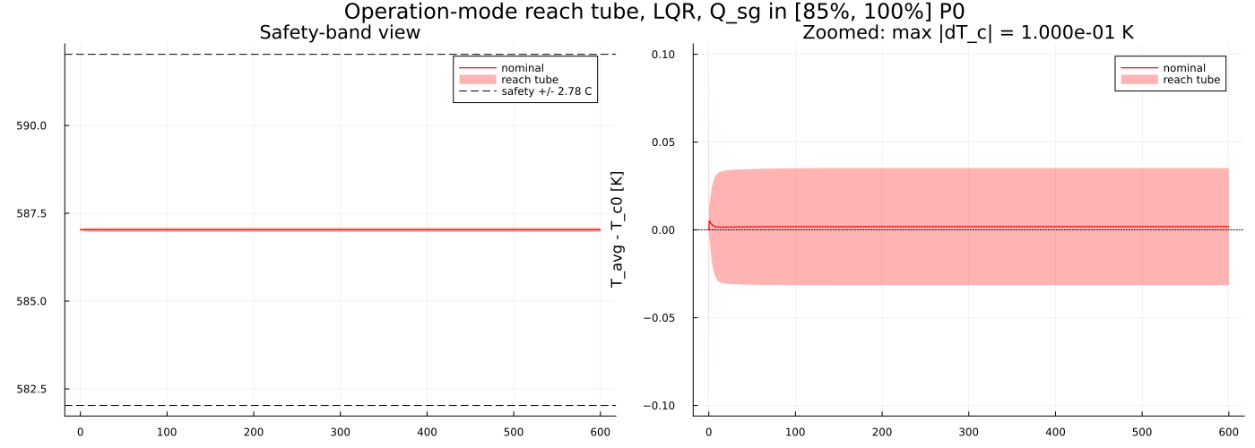
Operation-mode reach (under LQR) — discharges all 6 safety halfspaces

Reach tube starting from |dx_i| ≤ delta_entry, with Q_sg ∈ [85%, 100%] P_0 over 600 s. Per-halfspace result:

halfspace	headroom	reach-tube max	margin
fuel_centerline (T_f ≤ 1200 °C)	871.7 K	328.9	+871.1 ✓
t_avg_high_trip (T_c ≤ 320 °C)	11.6 K	308.4	+11.6 ✓
t_avg_low_trip (T_c ≥ 280 °C)	28.3 K	308.2	+28.2 ✓
n_high_trip (n ≤ 1.15)	0.150	1.012	+0.138 ✓
n_low_operation (n ≥ 0.15)	0.850	0.842	+0.692 ✓
cold_leg_subcooled (T_cold ≤ 305 °C)	15.0 K	292.9	+12.1 ✓

Tightest direction is n_high_trip — LQR lets n swing up to 1.012 to compensate for load swing, about 12% from the high-flux trip. All temperatures have 10-870 K margin.

Per-state reach-set width evolution over 600 s:

state	init halfwidth	final halfwidth	ratio
n	0.010	0.083	8.3× expand
C1..C6	varies	varies	160-200× expand
T_f	0.1 K	2.08 K	21× expand
T_c	0.1 K	0.033 K	0.33× contract
T_cold	0.1 K	1.47 K	15× expand

T_c contracts, everything else expands. This is the signature of good control: the regulated direction shrinks, unregulated directions drift. Precursors expand 200× but don't matter for safety (no predicate uses them).

Visualization (docs/figures/reach_operation_Tc.png):

Lyapunov barrier — fails all 6 safety halfspaces

Even with LQR and a Qbar sweep for the best quadratic weight:

halfspace	headroom	barrier max	margin
fuel_centerline	871.7	2244.1	-1372 ✗
t_avg_high_trip	11.6	33.3	-21.6 ✗
n_high_trip	0.150	1242	-1242 ✗
cold_leg_subcooled	15.0	150.7	-135.7 ✗

The barrier's ellipsoid says n could deviate by ±1242 — physically meaningless. That's closed-loop (LQR included); open-loop version is ±27 million. LQR helps by ~20,000× but the quadratic ellipsoid is fundamentally too coarse a geometry for this slab-shaped safety spec.

The anisotropy cost: Λ = 10⁻⁴ vs thermal timescales ~ seconds means any P solving the Lyapunov equation is ill-conditioned by 4 orders of magnitude. The resulting ellipsoid stretches absurdly in the fast directions (n, T_f) when projected to physical coordinates.

This is the motivation for SOS / polytopic barriers in the thesis: a quantitative, per-halfspace demonstration that quadratic Lyapunov is insufficient here, with the open-loop-vs-closed-loop comparison showing it's a structural issue not a tuning one.

Heatup mode — simulation only, no reach yet

The main_mode_sweep.m heatup scenario drives the plant from hot standby through the operating temperature:

Controller tracks the 28 °C/hr ramp with ~2 °F lag and ~5 °F final overshoot. Peak rate during ramp is 48.5 °C/hr (verified by plant-model/test_heatup_rate.m), right at the 50 °C/hr placeholder invariant but 70% over the nominal tech-spec rate. A strict 28 °C/hr invariant would be violated by the current controller tuning.

No linear heatup reach has been computed because:

1. The reference is time-varying — T_ref(t) = T_standby + rate·t. LQR around x_op doesn't apply; we'd need trajectory-LQR or linearization around a moving operating point (LTV reach).
2. Saturation sat(u) is active during early ramp — turns the controller into a hybrid sub-mode that linear reach can't handle without explicit region decomposition.
3. Even after feedback linearization, dn/dt is bilinear in (n, e).

Nonlinear reach (CORA or JuliaReach TMJets) is the right tool and is next on the list.

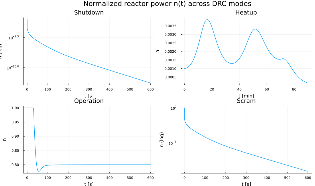
Other modes (sim only, no reach)

• Shutdown: holds cleanly. n: 1e-6 → 1e-12 over 10 min, temps flat. Reach would be trivial (constant u).
• Scram: n: 1 → 1e-6 over 10 min via prompt jump + delayed-neutron tail. Temp relaxes to ~379 °F at 3%-decay-heat balance. Reach obligation is bounded-time-to-subcritical; needs its own artifact.

Power overview:

---

5. Caveats, gaps, and next steps

Soundness status

The current reach tube is approximate, not sound, for the nonlinear plant.

reach_linear.m produces a sound over-approximation of the linearized closed-loop system's reach set. The linear model approximates the nonlinear plant with an error that is bounded but not currently computed or propagated into the tube. Two paths to soundness:

1. Nonlinear reach directly — CORA nonlinearSys (MATLAB) or ReachabilityAnalysis.jl Taylor models (TMJets, Julia). Expensive, honest.
2. Linear reach + Taylor-remainder inflation — compute an upper bound on ||f_nonlinear(x,u) - (Ax + Bu)|| over the reach set (via Hessian norm estimates per component) and inflate the linear tube. Cheaper, still rigorous.

For the thesis safety claim, either is required. The 28× margin of the linear tube gives us buffer to absorb linearization error but that's vibes, not a proof.

What's not modeled

• α drift (burnup, boron, xenon). The feedback-linearization in ctrl_heatup assumes exact α_f, α_c; real plants see α vary ~20% (burnup), ~10× (boron dilution), plus xenon transients. Robust treatment = α as an interval, propagate parametric uncertainty through reach.
• Saturation as hybrid sub-mode. ctrl_heatup saturates u; this is formally a 3-mode PWA system. Operation-mode LQR is dormant (trivially); heatup requires explicit region decomposition or dormancy proof.
• DNBR. inv1_holds and inv2_holds include fuel / temperature / power limits but not DNBR (departure from nucleate boiling ratio). DNBR needs a correlation (W-3, EPRI) that isn't modeled. Would add as a predicate DNBR(x) ≥ 1.3 once a correlation is selected.
• Cold shutdown. Plant model's α_f, α_c are linearized at HFP. True cold shutdown (~50 °C) is outside the model's ±50 °C trust region. "Shutdown" here = hot standby.
• Pressure / phase. c_c is constant; real cooldown drops pressure and changes water properties (IAPWS-IF97 lookups).
• Decay heat. n ≈ 0 doesn't capture residual fission-product heat. Wilson-Hardy correlation would add this if we go to real cold shutdown.

What's next

1. Nonlinear reach on heatup via JuliaReach — partial result in. ../julia-port/scripts/reach_heatup_nonlinear.jl ran successfully to T=10 s on the full 10-state nonlinear closed-loop (saturation disabled). Got 10,583 reach-sets with envelope T_c ∈ [274.45, 295] and n ∈ [-5e-4, 5e-3]. Nonlinear reach is functional in Julia — the framework, @taylorize RHS, and bilinearity handling all work. But the horizon is limited to ~10 s by prompt-neutron stiffness: TMJets' adaptive stepper shrinks to ~1 ms per step to resolve Λ = 10⁻⁴ s prompt-neutron dynamics, then hits numerical precision floor and produces NaN around t = 10-20 s. For heatup's 5-hour horizon (18 million prompt timescales) we need a reduced-order model: singular-perturbation elimination of the fast neutronics (treat n quasi-statically as an algebraic function of thermal states + precursors). Standard in reactor-kinetics reach literature. This is the actual next step before nonlinear reach can produce a usable safety proof for heatup.
2. Once nonlinear reach works: add saturation as hybrid sub-mode.
3. Parametric α reach once the framework can handle it.
4. Shutdown and scram reach (trivial cases, should be quick once the pattern is clear).
5. Pin mode boundaries to actual tech-spec numbers before defense. Currently they're engineering-reasonable-but-made-up.

The working mental model

• Linear reach artifacts here are design-validation + gut-check, not safety proofs. The 28× margin between the LQR reach tube and the safety halfspaces is the evidence that the controller probably works. Nonlinear reach converts this into an actual proof.
• The Lyapunov barrier fails on this plant and it's not a bug — it's the canonical tool's anisotropy limitation, demonstrated quantitatively. The thesis chapter should frame polytopic or SOS barriers as necessary, with the quadratic failure as the motivation.
• Per-mode reach obligations differ. Operation is disturbance rejection; heatup and scram are reach-avoid with time budgets; shutdown is trivial forever-invariance.